In-class_Ex02

Show the code

pacman::p_load(sf, tidyverse, funModeling)

3.1 Importing Geospatial

Your turn

Using the steps you had learned, import the LGA boundary GIS data of Nigeria downloaded from both sources recommended above.

3.1.1 The geoBoundaries data set

#| code-fold: true
#| code-summary: "Show the code"

geoNGA <- st_read("data/geospatial/",
                  layer =
                    "geoBoundaries-NGA-ADM2") %>%
  st_transform(crs = 26392)

Reading layer `geoBoundaries-NGA-ADM2' from data source 
  `C:\michellefaithl\is415-gaa-michellefaith\In-class_Ex\In-class_ex02\data\geospatial' 
  using driver `ESRI Shapefile'
Simple feature collection with 774 features and 6 fields
Geometry type: MULTIPOLYGON
Dimension:     XY
Bounding box:  xmin: 2.668534 ymin: 4.273007 xmax: 14.67882 ymax: 13.89442
Geodetic CRS:  WGS 84

The NGA data set

NGA <- st_read("data/geospatial/",
               layer = "nga_admbnda_adm2_osgof_20190417") %>%
  st_transform(crs = 26392)

Reading layer `nga_admbnda_adm2_osgof_20190417' from data source 
  `C:\michellefaithl\is415-gaa-michellefaith\In-class_Ex\In-class_ex02\data\geospatial' 
  using driver `ESRI Shapefile'
Simple feature collection with 774 features and 16 fields
Geometry type: MULTIPOLYGON
Dimension:     XY
Bounding box:  xmin: 2.668534 ymin: 4.273007 xmax: 14.67882 ymax: 13.89442
Geodetic CRS:  WGS 84

Show the code

wp_nga <- read_csv("data/aspatial/WPdx.csv") %>%
  filter(`#clean_country_name` == "Nigeria")

Warning: One or more parsing issues, call `problems()` on your data frame for details,
e.g.:
  dat <- vroom(...)
  problems(dat)

Rows: 406566 Columns: 70
── Column specification ────────────────────────────────────────────────────────
Delimiter: ","
chr (43): #source, #report_date, #status_id, #water_source_clean, #water_sou...
dbl (23): row_id, #lat_deg, #lon_deg, #install_year, #fecal_coliform_value, ...
lgl  (4): #rehab_year, #rehabilitator, is_urban, latest_record

ℹ Use `spec()` to retrieve the full column specification for this data.
ℹ Specify the column types or set `show_col_types = FALSE` to quiet this message.

3.2 Importing

Converting water point data into sf point features

Converting an aspatial data into an sf data.frame

Show the code

wp_nga$Geometry = st_as_sfc(wp_nga$'New Georeferenced Column')
wp_nga

# A tibble: 95,008 × 71
   row_id `#source`      #lat_…¹ #lon_…² #repo…³ #stat…⁴ #wate…⁵ #wate…⁶ #wate…⁷
    <dbl> <chr>            <dbl>   <dbl> <chr>   <chr>   <chr>   <chr>   <chr>  
 1 429068 GRID3             7.98    5.12 08/29/… Unknown <NA>    <NA>    Tapsta…
 2 222071 Federal Minis…    6.96    3.60 08/16/… Yes     Boreho… Well    Mechan…
 3 160612 WaterAid          6.49    7.93 12/04/… Yes     Boreho… Well    Hand P…
 4 160669 WaterAid          6.73    7.65 12/04/… Yes     Boreho… Well    <NA>   
 5 160642 WaterAid          6.78    7.66 12/04/… Yes     Boreho… Well    Hand P…
 6 160628 WaterAid          6.96    7.78 12/04/… Yes     Boreho… Well    Hand P…
 7 160632 WaterAid          7.02    7.84 12/04/… Yes     Boreho… Well    Hand P…
 8 642747 Living Water …    7.33    8.98 10/03/… Yes     Boreho… Well    Mechan…
 9 642456 Living Water …    7.17    9.11 10/03/… Yes     Boreho… Well    Hand P…
10 641347 Living Water …    7.20    9.22 03/28/… Yes     Boreho… Well    Hand P…
# … with 94,998 more rows, 62 more variables: `#water_tech_category` <chr>,
#   `#facility_type` <chr>, `#clean_country_name` <chr>, `#clean_adm1` <chr>,
#   `#clean_adm2` <chr>, `#clean_adm3` <chr>, `#clean_adm4` <chr>,
#   `#install_year` <dbl>, `#installer` <chr>, `#rehab_year` <lgl>,
#   `#rehabilitator` <lgl>, `#management_clean` <chr>, `#status_clean` <chr>,
#   `#pay` <chr>, `#fecal_coliform_presence` <chr>,
#   `#fecal_coliform_value` <dbl>, `#subjective_quality` <chr>, …

Show the code

wp_sf <- st_sf(wp_nga, crs=4326)
wp_sf

Simple feature collection with 95008 features and 70 fields
Geometry type: POINT
Dimension:     XY
Bounding box:  xmin: 2.707441 ymin: 4.301812 xmax: 14.21828 ymax: 13.86568
Geodetic CRS:  WGS 84
# A tibble: 95,008 × 71
   row_id `#source`      #lat_…¹ #lon_…² #repo…³ #stat…⁴ #wate…⁵ #wate…⁶ #wate…⁷
 *  <dbl> <chr>            <dbl>   <dbl> <chr>   <chr>   <chr>   <chr>   <chr>  
 1 429068 GRID3             7.98    5.12 08/29/… Unknown <NA>    <NA>    Tapsta…
 2 222071 Federal Minis…    6.96    3.60 08/16/… Yes     Boreho… Well    Mechan…
 3 160612 WaterAid          6.49    7.93 12/04/… Yes     Boreho… Well    Hand P…
 4 160669 WaterAid          6.73    7.65 12/04/… Yes     Boreho… Well    <NA>   
 5 160642 WaterAid          6.78    7.66 12/04/… Yes     Boreho… Well    Hand P…
 6 160628 WaterAid          6.96    7.78 12/04/… Yes     Boreho… Well    Hand P…
 7 160632 WaterAid          7.02    7.84 12/04/… Yes     Boreho… Well    Hand P…
 8 642747 Living Water …    7.33    8.98 10/03/… Yes     Boreho… Well    Mechan…
 9 642456 Living Water …    7.17    9.11 10/03/… Yes     Boreho… Well    Hand P…
10 641347 Living Water …    7.20    9.22 03/28/… Yes     Boreho… Well    Hand P…
# … with 94,998 more rows, 62 more variables: `#water_tech_category` <chr>,
#   `#facility_type` <chr>, `#clean_country_name` <chr>, `#clean_adm1` <chr>,
#   `#clean_adm2` <chr>, `#clean_adm3` <chr>, `#clean_adm4` <chr>,
#   `#install_year` <dbl>, `#installer` <chr>, `#rehab_year` <lgl>,
#   `#rehabilitator` <lgl>, `#management_clean` <chr>, `#status_clean` <chr>,
#   `#pay` <chr>, `#fecal_coliform_presence` <chr>,
#   `#fecal_coliform_value` <dbl>, `#subjective_quality` <chr>, …

Transforming into Nigeria projected coordinate system

Show the code

wp_sf <- wp_sf %>%
  st_transform(crs = 26392)

4 Geospatial Data

Excluding redundant fields

Show the code

NGA <- NGA %>% 
  select (c(3:4, 8:9))

Checking for duplicate name

It is always important to check for duplicate name in the data in the data main data fields. Using duplicated() of Base R, we can flag out LGA names that might be duplicated as shown in the code chunk below.

NGA$ADN2_EN[duplicated(NGA$ADM2_EN)==TRUE]

NULL

Let us correct these errors by using the code chunk below.

NGA$ADM2_EN[94] <- "Bassa, Kogi"
NGA$ADM2_EN[95] <- "Bassa, Plateau"
NGA$ADM2_EN[304] <- "Ifelodun, Kwara"
NGA$ADM2_EN[305] <- "Ifelodun, Osun"
NGA$ADM2_EN[355] <- "Irepodun, Kwara"
NGA$ADM2_EN[356] <- "Irepodun, Osun"
NGA$ADM2_EN[519] <- "Nasarawa, Kano"
NGA$ADM2_EN[520] <- "Nasarawa, Nasarawa"
NGA$ADM2_EN[546] <- "Obi, Benue"
NGA$ADM2_EN[547] <- "Obi, Nasarawa"
NGA$ADM2_EN[693] <- "Surulere, Lagos"
NGA$ADM2_EN[694] <- "Surulere, Oyo"

Let us check again if there is any duplicates. ::: {style=“font-size: 1.2em”}

NGA$ADN2_EN[duplicated(NGA$ADM2_EN)==TRUE]

NULL

:::

5 Data Wrangling for Water Point Data

freq(data = wp_sf,
     input = '#status_clean')

Warning: The `<scale>` argument of `guides()` cannot be `FALSE`. Use "none" instead as
of ggplot2 3.3.4.
ℹ The deprecated feature was likely used in the funModeling package.
  Please report the issue at <https://github.com/pablo14/funModeling/issues>.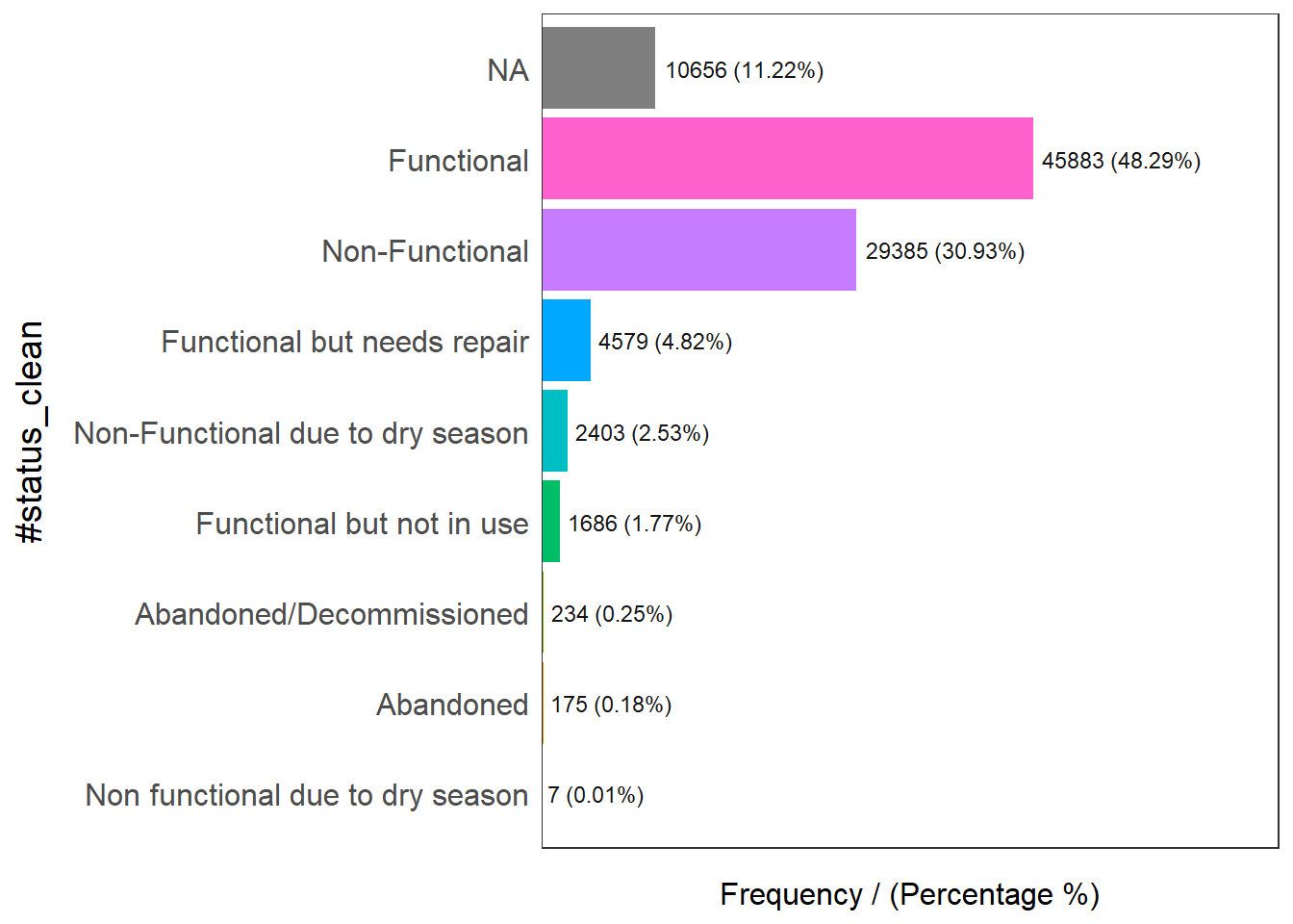

                     #status_clean frequency percentage cumulative_perc
1                       Functional     45883      48.29           48.29
2                   Non-Functional     29385      30.93           79.22
3                             <NA>     10656      11.22           90.44
4      Functional but needs repair      4579       4.82           95.26
5 Non-Functional due to dry season      2403       2.53           97.79
6        Functional but not in use      1686       1.77           99.56
7         Abandoned/Decommissioned       234       0.25           99.81
8                        Abandoned       175       0.18           99.99
9 Non functional due to dry season         7       0.01          100.00

Rename NA to unknown. ::: {style=“font-size: 1.2em”}

wp_sf_nga <- wp_sf %>%
  rename(status_clean = '#status_clean') %>%
  select(status_clean) %>%
  mutate(status_clean = replace_na(
    status_clean, "unknown"))

:::

Extracting Water Point Data

Now we are ready to extract the water point daa according to their status.

The code chunk below is used to extract functional water point.

wp_functional <- wp_sf_nga %>%
  filter(status_clean %in%
           c("Functional",
             "Functional but not in use",
             "Functional but needs repair"))

The code chunk below is used to extract nonfunctional water point.

wp_nonfunctional <- wp_sf_nga %>%
  filter(status_clean %in%
           c("Abandoned/Decommissioned",
             "Abandoned",
             "Non-Functional due to dry season",
             "Non-Functional",
             "Non functional due to dry season"))

The code chunk below is used to extract water point ::: {style=“font-size: 1.2em”}

wp_unknown <- wp_sf_nga %>%
  filter(status_clean == "unknown")

:::

Performing Point-in-Polygon Count

NGA_wp <- NGA %>%
  mutate (`total_wp` = lengths(
    st_intersects(NGA, wp_sf_nga))) %>%
  mutate (`wp_functional` = lengths(
    st_intersects(NGA, wp_functional))) %>%
  mutate (`wp_nonfunctional` = lengths(
    st_intersects(NGA, wp_nonfunctional))) %>%
  mutate (`wp_unknown` = lengths(
    st_intersects(NGA, wp_unknown))) 

Saving the analytical data in rds format

In order to retain the sf object structure for subsequent analysis, it is recommended to save the sf data.frame into rds format.

In the code chunk below, write_rds() of readr package is used to export an sf data.frame into rds format.

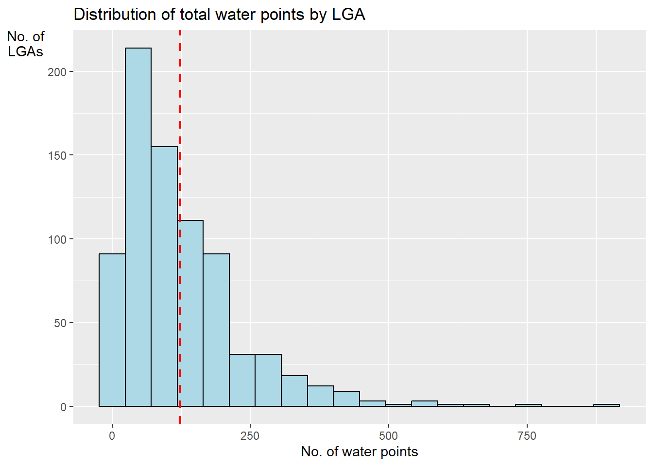
write_rds(NGA_wp, "data/rds/NGA_WP.rds")

Visualising attributes by using statistical graphs

ggplot(data = NGA_wp,
       aes(x = total_wp)) +
  geom_histogram(bins=20, color="black",
                 fill="light blue") +
  geom_vline(aes(xintercept=mean(
    total_wp, na.rm=T  )),
              color = "red",
              linetype="dashed",
              size=0.8) +
  ggtitle("Distribution of total water points by LGA") +
  xlab("No. of water points") +
  ylab("No. of\nLGAs") +
  theme(axis.title.y=element_text(angle=0))

Warning: Using `size` aesthetic for lines was deprecated in ggplot2 3.4.0.
ℹ Please use `linewidth` instead.