pacman::p_load(tidyverse, tmap, sf, sfdep, plotly)In-class_Ex07: Global and Local Measures of Spatial Association - sfdep methods
Getting Started
Importing Data
hunan <- st_read(dsn = "data/geospatial",
                     layer = "Hunan")
Reading layer `Hunan' from data source
`C:\michellefaithl\is415-gaa-michellefaith\In-class_Ex\In-class_ex07\data\geospatial'
using driver `ESRI Shapefile'
Simple feature collection with 88 features and 7 fields
Geometry type: POLYGON
Dimension: XY
Bounding box: xmin: 108.7831 ymin: 24.6342 xmax: 114.2544 ymax: 30.12812
Geodetic CRS: WGS 84hunan2012 <- read_csv("data/aspatial/Hunan_2012.csv")Joining using left join
hunan_GDPPC <- left_join(hunan, hunan2012) %>%
  select(1:4, 7, 15)
Deriving contiguity weights: queen’s method
wm_q <- hunan_GDPPC %>%
  mutate(nb = st_contiguity(geometry),
         wt = st_weights(nb,
                         style = "W"),
         .before = 1)
computing global moran’ I
moranI <- global_moran(wm_q$GDPPC,
                       wm_q$nb,
                       wm_q$wt)
performing gloabl moran’I test
global_moran_test(wm_q$GDPPC,
                  wm_q$nb,
                  wm_q$wt)
    Moran I test under randomisation

data:  x
weights: listw

Moran I statistic standard deviate = 4.7351, p-value = 1.095e-06
alternative hypothesis: greater
sample estimates:
Moran I statistic       Expectation          Variance
0.300749970 -0.011494253 0.004348351 set.seed(1234)global_moran_perm(wm_q$GDPPC,
wm_q$nb,
wm_q$wt,
nsim = 99)
    Monte-Carlo simulation of Moran I

data:  x
weights: listw
number of simulations + 1: 100

statistic = 0.30075, observed rank = 100, p-value < 2.2e-16
alternative hypothesis: two.sided
Computing local Moran’s I
lisa <- wm_q %>%
  mutate(local_moran= local_moran(
    GDPPC, nb, wt, nsim = 99),
      .before = 1) %>%
  unnest(local_moran)
lisa
Simple feature collection with 88 features and 20 fields
Geometry type: POLYGON
Dimension: XY
Bounding box: xmin: 108.7831 ymin: 24.6342 xmax: 114.2544 ymax: 30.12812
Geodetic CRS: WGS 84
# A tibble: 88 × 21
ii eii var_ii z_ii p_ii p_ii_…¹ p_fol…² skewn…³ kurtosis
<dbl> <dbl> <dbl> <dbl> <dbl> <dbl> <dbl> <dbl> <dbl>
1 -0.00147 0.00177 4.18e-4 -0.158 0.874 0.82 0.41 -0.812 0.652
2 0.0259 0.00641 1.05e-2 0.190 0.849 0.96 0.48 -1.09 1.89
3 -0.0120 -0.0374 1.02e-1 0.0796 0.937 0.76 0.38 0.824 0.0461
4 0.00102 -0.0000349 4.37e-6 0.506 0.613 0.64 0.32 1.04 1.61
5 0.0148 -0.00340 1.65e-3 0.449 0.654 0.5 0.25 1.64 3.96
6 -0.0388 -0.00339 5.45e-3 -0.480 0.631 0.82 0.41 0.614 -0.264
7 3.37 -0.198 1.41e+0 3.00 0.00266 0.08 0.04 1.46 2.74
8 1.56 -0.265 8.04e-1 2.04 0.0417 0.08 0.04 0.459 -0.519
9 4.42 0.0450 1.79e+0 3.27 0.00108 0.02 0.01 0.746 -0.00582
10 -0.399 -0.0505 8.59e-2 -1.19 0.234 0.28 0.14 -0.685 0.134
# … with 78 more rows, 12 more variables: mean <fct>, median <fct>,
# pysal <fct>, nb <nb>, wt <list>, NAME_2 <chr>, ID_3 <int>, NAME_3 <chr>,
# ENGTYPE_3 <chr>, County <chr>, GDPPC <dbl>, geometry <POLYGON [°]>, and
# abbreviated variable names ¹p_ii_sim, ²p_folded_sim, ³skewnessvisualising local Moran’s I
tmap_mode("plot")
tm_shape(lisa) +
  tm_fill("ii") +
  tm_borders(alpha = 0.5) +
  tm_view(set.zoom.limits = c(6,8))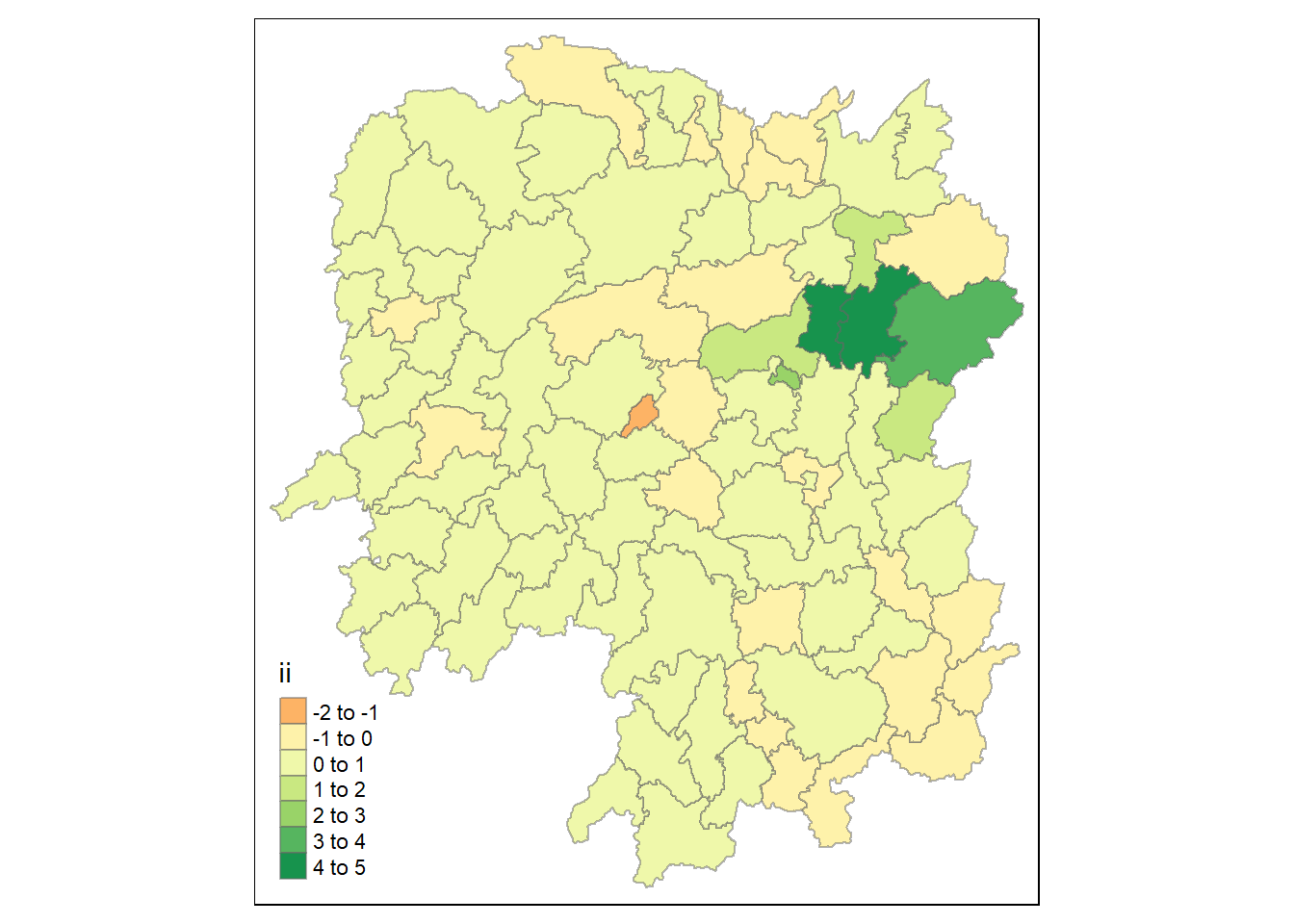
tmap_mode("plot")
tm_shape(lisa) +
  tm_fill("p_ii_sim") +
  tm_borders(alpha = 0.5)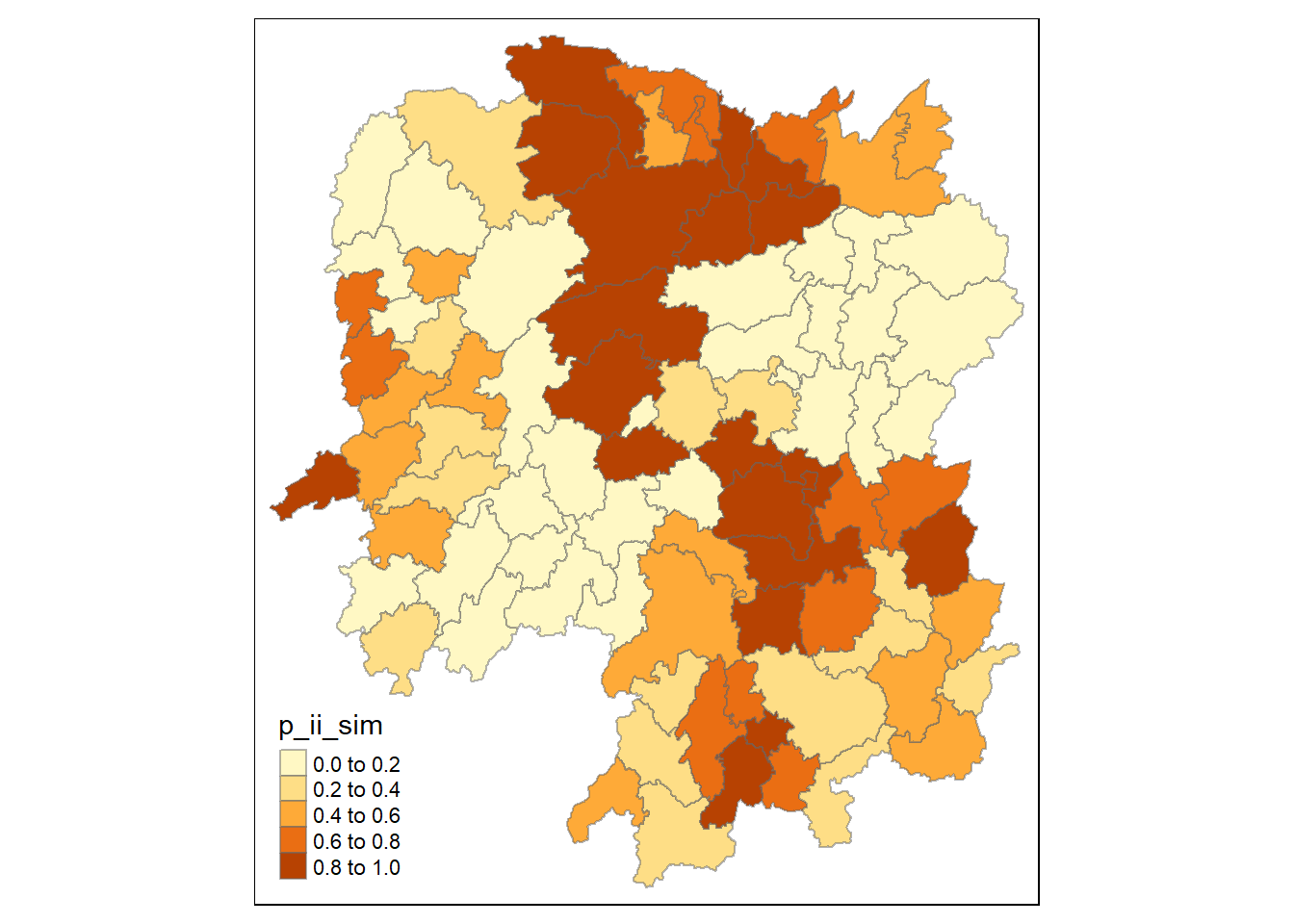
lisa_sig <- lisa %>%
  filter(p_ii < 0.05)
tmap_mode("plot")
tm_shape(lisa) +
  tm_polygons() +
  tm_borders(alpha = 0.5) +
  tm_shape(lisa_sig) +
  tm_fill("mean") +
tm_borders(alpha = 0.4) 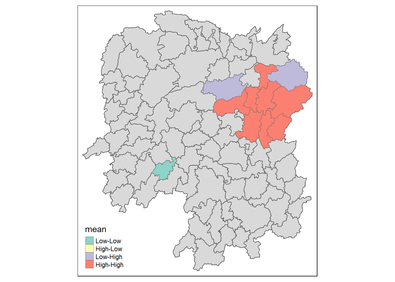
computing local Moran’s I
HCSA <- wm_q %>%
  mutate(local_Gi = local_gstar_perm(
    GDPPC, nb, nsim = 99),
      .before = 1) %>%
  unnest(local_Gi)
HCSA
Simple feature collection with 88 features and 16 fields
Geometry type: POLYGON
Dimension: XY
Bounding box: xmin: 108.7831 ymin: 24.6342 xmax: 114.2544 ymax: 30.12812
Geodetic CRS: WGS 84
# A tibble: 88 × 17
gi_star e_gi var_gi p_value p_sim p_fol…¹ skewn…² kurto…³ nb wt
<dbl> <dbl> <dbl> <dbl> <dbl> <dbl> <dbl> <dbl> <nb> <lis>
1 -0.00567 0.0115 0.00000812 9.95e-1 0.82 0.41 1.03 1.23 <int> <dbl>
2 -0.235 0.0110 0.00000581 8.14e-1 1 0.5 0.912 1.05 <int> <dbl>
3 0.298 0.0114 0.00000776 7.65e-1 0.7 0.35 0.455 -0.732 <int> <dbl>
4 0.145 0.0121 0.0000111 8.84e-1 0.64 0.32 0.900 0.726 <int> <dbl>
5 0.356 0.0113 0.0000119 7.21e-1 0.64 0.32 1.08 1.31 <int> <dbl>
6 -0.480 0.0116 0.00000706 6.31e-1 0.82 0.41 0.364 -0.676 <int> <dbl>
7 3.66 0.0116 0.00000825 2.47e-4 0.02 0.01 0.909 0.664 <int> <dbl>
8 2.14 0.0116 0.00000714 3.26e-2 0.16 0.08 1.13 1.48 <int> <dbl>
9 4.55 0.0113 0.00000656 5.28e-6 0.02 0.01 1.36 4.14 <int> <dbl>
10 1.61 0.0109 0.00000341 1.08e-1 0.18 0.09 0.269 -0.396 <int> <dbl>
# … with 78 more rows, 7 more variables: NAME_2 <chr>, ID_3 <int>,
# NAME_3 <chr>, ENGTYPE_3 <chr>, County <chr>, GDPPC <dbl>,
# geometry <POLYGON [°]>, and abbreviated variable names ¹p_folded_sim,
# ²skewness, ³kurtosisHot Spot and Cold Spot Area Analysis (HCSA)
HCSA uses spatial weights to identify locations of statistically significant hot spots and cold spots in an spatially weighted attribute that are in proximity to one another based on a calculated distance. The analysis groups features when similar high (hot) or low (cold) values are found in a cluster. The polygon features usually represent administration boundaries or a custom grid structure.
Computing local Gi* statistics
wm_idw <- hunan_GDPPC %>%
  mutate(nb = st_contiguity(geometry),
         wts = st_inverse_distance(nb, geometry,
                                   scale = 1,
                                   alpha = 1),
         .before = 1)
HCSA <- wm_idw %>%
mutate(local_Gi = local_gstar_perm(
GDPPC, nb, wt, nsim = 99),
.before = 1) %>%
unnest(local_Gi)
HCSASimple feature collection with 88 features and 16 fields
Geometry type: POLYGON
Dimension: XY
Bounding box: xmin: 108.7831 ymin: 24.6342 xmax: 114.2544 ymax: 30.12812
Geodetic CRS: WGS 84
# A tibble: 88 × 17
gi_star e_gi var_gi p_value p_sim p_fol…¹ skewn…² kurto…³ nb wts
<dbl> <dbl> <dbl> <dbl> <dbl> <dbl> <dbl> <dbl> <nb> <lis>
1 0.243 0.0108 0.00000807 8.08e-1 0.54 0.27 1.40 2.08 <int> <dbl>
2 -0.434 0.0119 0.0000112 6.64e-1 0.82 0.41 0.779 0.0896 <int> <dbl>
3 0.400 0.0111 0.00000803 6.89e-1 0.68 0.34 0.766 -0.130 <int> <dbl>
4 0.156 0.0120 0.0000130 8.76e-1 0.78 0.39 1.22 2.12 <int> <dbl>
5 0.476 0.0111 0.00000858 6.34e-1 0.58 0.29 1.15 1.43 <int> <dbl>
6 0.00786 0.0103 0.00000505 9.94e-1 0.9 0.45 0.648 -0.171 <int> <dbl>
7 4.24 0.0108 0.00000724 2.25e-5 0.02 0.01 0.721 0.225 <int> <dbl>
8 2.89 0.0110 0.00000482 3.82e-3 0.04 0.02 0.743 0.864 <int> <dbl>
9 5.87 0.0105 0.00000450 4.43e-9 0.02 0.01 0.783 0.375 <int> <dbl>
10 1.21 0.0114 0.00000417 2.25e-1 0.26 0.13 0.705 0.403 <int> <dbl>
# … with 78 more rows, 7 more variables: NAME_2 <chr>, ID_3 <int>,
# NAME_3 <chr>, ENGTYPE_3 <chr>, County <chr>, GDPPC <dbl>,
# geometry <POLYGON [°]>, and abbreviated variable names ¹p_folded_sim,
# ²skewness, ³kurtosis