#pacman::p_load(tmap, tidyverse, sf, funModeling, sfdep, raster)
pacman::p_load(tmap, tidyverse, sf, funModeling, sfdep)Take-home Exercise 1: Application of Spatial Point Patterns Analysis to discover the geographical distribution of functional and non-function water points in Osub State, Nigeria
1 Overview
1.1 Setting the Scene
Water is an important resource to mankind. Clean and accessible water is critical to human health. It provides a healthy environment, a sustainable economy, reduces poverty and ensures peace and security. Yet over 40% of the global population does not have access to sufficient clean water. By 2025, 1.8 billion people will be living in countries or regions with absolute water scarcity, according to UN-Water. The lack of water poses a major threat to several sectors, including food security. Agriculture uses about 70% of the world’s accessible freshwater.
Developing countries are most affected by water shortages and poor water quality. Up to 80% of illnesses in the developing world are linked to inadequate water and sanitation. Despite technological advancement, providing clean water to the rural community is still a major development issues in many countries globally, especially countries in the Africa continent.
To address the issue of providing clean and sustainable water supply to the rural community, a global Water Point Data Exchange (WPdx) project has been initiated. The main aim of this initiative is to collect water point related data from rural areas at the water point or small water scheme level and share the data via WPdx Data Repository, a cloud-based data library. What is so special of this project is that data are collected based on WPDx Data Standard.
1.2 Objectives
Geospatial analytics hold tremendous potential to address complex problems facing society. In this study, you are tasked to apply appropriate spatial point patterns analysis methods to discover the geographical distribution of functional and non-function water points and their co-locations if any in Osun State, Nigeria.
1.3 The Data
1.3.1 Aspatial Data
For the purpose of this assignment, data from WPdx Global Data Repositories will be used. There are two versions of the data. They are: WPdx-Basic and WPdx+. You are required to use WPdx+ data set.
1.3.2 Spatial Data
Nigeria Level-2 Administrative Boundary (also known as Local Government Area) polygon features GIS data will be used in this take-home exercise. The data can be downloaded either from The Humanitarian Data Exchange portal or geoBoundaries.
1.4 The Task
The specific tasks of this take-home exercise are as follows:
Exploratory Spatial Data Analysis (ESDA)
Derive kernel density maps of functional and non-functional water points. Using appropriate tmap functions,
Display the kernel density maps on openstreetmap of Osub State, Nigeria. Describe the spatial patterns revealed by the kernel density maps.
Highlight the advantage of kernel density map over point map.
Second-order Spatial Point Patterns Analysis
With reference to the spatial point patterns observed in ESDA:
Formulate the null hypothesis and alternative hypothesis and select the confidence level.
Perform the test by using appropriate Second order spatial point patterns analysis technique.
With reference to the analysis results, draw statistical conclusions.
Spatial Correlation Analysis
In this section, you are required to confirm statistically if the spatial distribution of functional and non-functional water points are independent from each other.
Formulate the null hypothesis and alternative hypothesis and select the confidence level.
Perform the test by using appropriate Second order spatial point patterns analysis technique.
With reference to the analysis results, draw statistical conclusions.
2 Getting Started
The R packages we’ll use for this analysis are:
sf: used for importing, managing, and processing geospatial data
tidyverse: a collection of packages for data science tasks
tmap: used for creating thematic maps, such as choropleth and bubble maps
spatstat: used for point pattern analysis
raster: reads, writes, manipulates, analyses and models gridded spatial data (e.g. raster-based geographical data)
funModeling: covers common aspects in predictive modeling (e.g. data cleaning, variable importance analysis and assessing model performance)
sfdep: performing geospatial data wrangling and local colocation quotient analysis
maptools: maptools which provides a set of tools for manipulating geographic data. In this hands-on exercise, we mainly use it to convert Spatial objects into ppp format of spatstat.
3 Handling Geospatial Data
3.1 Importing Geospatial Data
We will be importing the following geospatial datasets in R by using st_read() of sf package:
The geoBoundaries Dataset
The NGA data set
3.1.1 The geoBoundaries Dataset
geoNGA <- st_read("data/geospatial/",
layer = "geoBoundaries-NGA-ADM2") %>%
st_transform(crs = 26392)Reading layer `geoBoundaries-NGA-ADM2' from data source
`C:\michellefaithl\is415-gaa-michellefaith\Take-home_Ex\data\geospatial'
using driver `ESRI Shapefile'
Simple feature collection with 774 features and 6 fields
Geometry type: MULTIPOLYGON
Dimension: XY
Bounding box: xmin: 2.668534 ymin: 4.273007 xmax: 14.67882 ymax: 13.89442
Geodetic CRS: WGS 843.1.2 The NGA Dataset
NGA <- st_read("data/geospatial/",
layer = "geoBoundaries-NGA-ADM2") %>%
st_transform(crs = 26392)Reading layer `geoBoundaries-NGA-ADM2' from data source
`C:\michellefaithl\is415-gaa-michellefaith\Take-home_Ex\data\geospatial'
using driver `ESRI Shapefile'
Simple feature collection with 774 features and 6 fields
Geometry type: MULTIPOLYGON
Dimension: XY
Bounding box: xmin: 2.668534 ymin: 4.273007 xmax: 14.67882 ymax: 13.89442
Geodetic CRS: WGS 84By examining both sf dataframe closely, we notice that NGA provide both LGA and state information. Hence, NGA data.frame will be used for the subsequent processing.
3.2 Importing Aspatial Data
We will use read_csv() of readr package to import only water points within Nigeria.
wp_nga <- read_csv("data/aspatial/WPdx.csv") %>%
filter(`#clean_country_name` == "Nigeria")3.2.1 Converting water point data into sf point features
Converting an aspatial data into an sf data.frame involves two steps.
First, we need to convert the wkt field into sfc field by using st_as_sfc() data type.
wp_nga$Geometry = st_as_sfc(wp_nga$`New Georeferenced Column`)
wp_nga# A tibble: 95,008 × 71
row_id `#source` #lat_…¹ #lon_…² #repo…³ #stat…⁴ #wate…⁵ #wate…⁶ #wate…⁷
<dbl> <chr> <dbl> <dbl> <chr> <chr> <chr> <chr> <chr>
1 429068 GRID3 7.98 5.12 08/29/… Unknown <NA> <NA> Tapsta…
2 222071 Federal Minis… 6.96 3.60 08/16/… Yes Boreho… Well Mechan…
3 160612 WaterAid 6.49 7.93 12/04/… Yes Boreho… Well Hand P…
4 160669 WaterAid 6.73 7.65 12/04/… Yes Boreho… Well <NA>
5 160642 WaterAid 6.78 7.66 12/04/… Yes Boreho… Well Hand P…
6 160628 WaterAid 6.96 7.78 12/04/… Yes Boreho… Well Hand P…
7 160632 WaterAid 7.02 7.84 12/04/… Yes Boreho… Well Hand P…
8 642747 Living Water … 7.33 8.98 10/03/… Yes Boreho… Well Mechan…
9 642456 Living Water … 7.17 9.11 10/03/… Yes Boreho… Well Hand P…
10 641347 Living Water … 7.20 9.22 03/28/… Yes Boreho… Well Hand P…
# … with 94,998 more rows, 62 more variables: `#water_tech_category` <chr>,
# `#facility_type` <chr>, `#clean_country_name` <chr>, `#clean_adm1` <chr>,
# `#clean_adm2` <chr>, `#clean_adm3` <chr>, `#clean_adm4` <chr>,
# `#install_year` <dbl>, `#installer` <chr>, `#rehab_year` <lgl>,
# `#rehabilitator` <lgl>, `#management_clean` <chr>, `#status_clean` <chr>,
# `#pay` <chr>, `#fecal_coliform_presence` <chr>,
# `#fecal_coliform_value` <dbl>, `#subjective_quality` <chr>, …Next, we will convert the tibble data.frame into an sf object by using st_sf(). It is also important for us to include the referencing system of the data into the sf object.
wp_sf <- st_sf(wp_nga, crs=4326)
wp_sfSimple feature collection with 95008 features and 70 fields
Geometry type: POINT
Dimension: XY
Bounding box: xmin: 2.707441 ymin: 4.301812 xmax: 14.21828 ymax: 13.86568
Geodetic CRS: WGS 84
# A tibble: 95,008 × 71
row_id `#source` #lat_…¹ #lon_…² #repo…³ #stat…⁴ #wate…⁵ #wate…⁶ #wate…⁷
* <dbl> <chr> <dbl> <dbl> <chr> <chr> <chr> <chr> <chr>
1 429068 GRID3 7.98 5.12 08/29/… Unknown <NA> <NA> Tapsta…
2 222071 Federal Minis… 6.96 3.60 08/16/… Yes Boreho… Well Mechan…
3 160612 WaterAid 6.49 7.93 12/04/… Yes Boreho… Well Hand P…
4 160669 WaterAid 6.73 7.65 12/04/… Yes Boreho… Well <NA>
5 160642 WaterAid 6.78 7.66 12/04/… Yes Boreho… Well Hand P…
6 160628 WaterAid 6.96 7.78 12/04/… Yes Boreho… Well Hand P…
7 160632 WaterAid 7.02 7.84 12/04/… Yes Boreho… Well Hand P…
8 642747 Living Water … 7.33 8.98 10/03/… Yes Boreho… Well Mechan…
9 642456 Living Water … 7.17 9.11 10/03/… Yes Boreho… Well Hand P…
10 641347 Living Water … 7.20 9.22 03/28/… Yes Boreho… Well Hand P…
# … with 94,998 more rows, 62 more variables: `#water_tech_category` <chr>,
# `#facility_type` <chr>, `#clean_country_name` <chr>, `#clean_adm1` <chr>,
# `#clean_adm2` <chr>, `#clean_adm3` <chr>, `#clean_adm4` <chr>,
# `#install_year` <dbl>, `#installer` <chr>, `#rehab_year` <lgl>,
# `#rehabilitator` <lgl>, `#management_clean` <chr>, `#status_clean` <chr>,
# `#pay` <chr>, `#fecal_coliform_presence` <chr>,
# `#fecal_coliform_value` <dbl>, `#subjective_quality` <chr>, …3.2.2 Transforming the Nigeria projected coordinate system
We will now transform the projection from wgs84 to an appropriate projected coordinate system of Nigeria.
wp_sf <- wp_sf %>%
st_transform(crs = 26392)4 Data Wrangling for Water Point Data
Exploratory Data Analysis (EDA) is a popular approach to gain initial understanding of the data. In the code chunk below, freq() of funModeling package is used to reveal the distribution of water point status visually.
freq(data = wp_sf,
input = '#status_clean')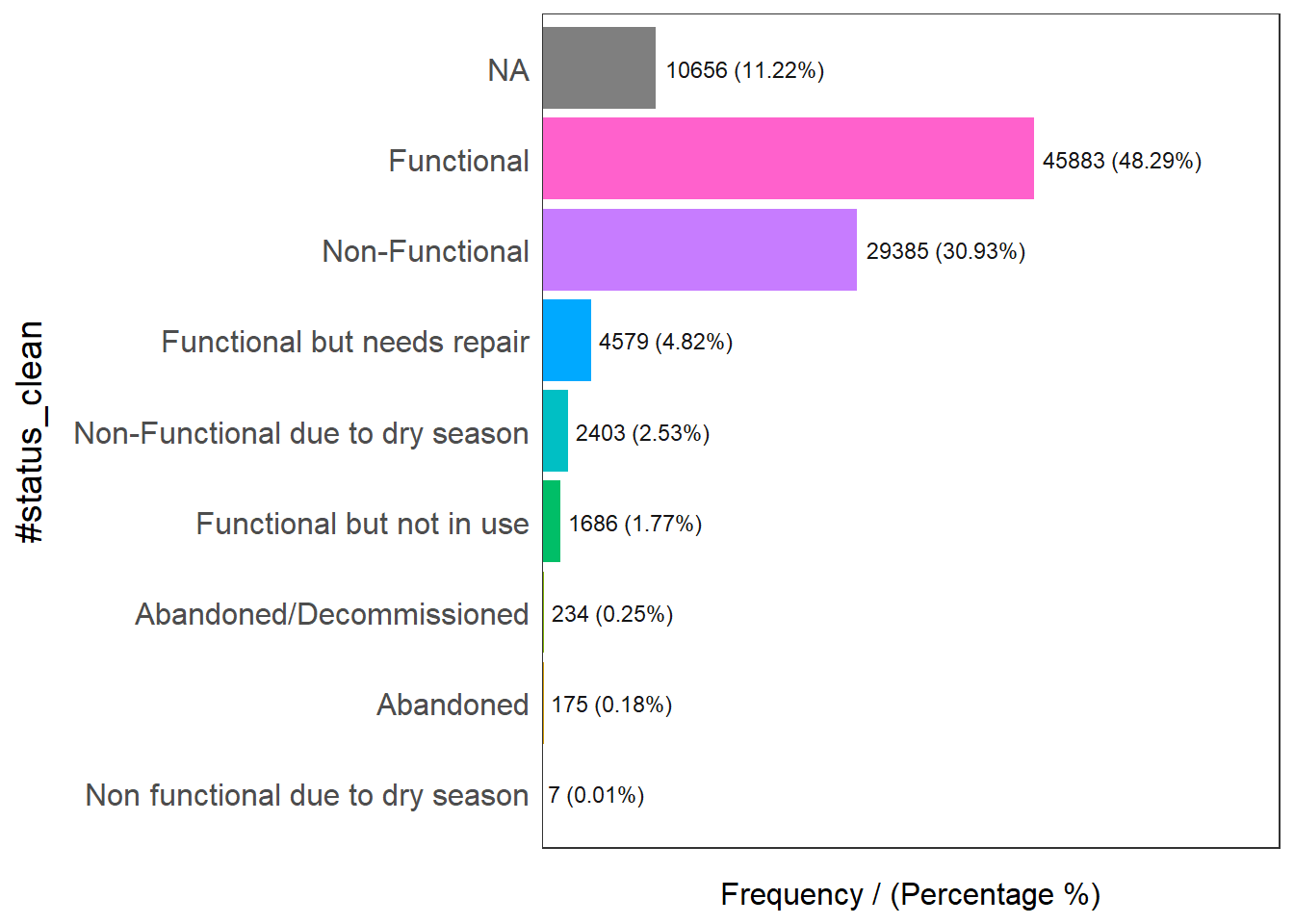
#status_clean frequency percentage cumulative_perc
1 Functional 45883 48.29 48.29
2 Non-Functional 29385 30.93 79.22
3 <NA> 10656 11.22 90.44
4 Functional but needs repair 4579 4.82 95.26
5 Non-Functional due to dry season 2403 2.53 97.79
6 Functional but not in use 1686 1.77 99.56
7 Abandoned/Decommissioned 234 0.25 99.81
8 Abandoned 175 0.18 99.99
9 Non functional due to dry season 7 0.01 100.00Figure above shows that there are nine classes in the #status_clean fields.
Next, code chunk below will be used to perform the following data wrangling tasksP - rename() of dplyr package is used to rename the column from #status_clean to status_clean for easier handling in subsequent steps. - select() of dplyr is used to include status_clean in the output sf data.frame. - mutate() and replace_na() are used to recode all the NA values in status_clean into unknown.
wp_sf_nga <- wp_sf %>%
rename(status_clean = '#status_clean') %>%
select(status_clean) %>%
mutate(status_clean = replace_na(
status_clean, "unknown"))4.1 Extracting Water Point Data
Now we are ready to extract the water point data according to their status.
The code chunk below is used to extract functional water point.
wp_functional <- wp_sf_nga %>%
filter(status_clean %in%
c("Functional",
"Functional but not in use",
"Functional but needs repair"))The code chunk below is used to extract nonfunctional water point.
wp_nonfunctional <- wp_sf_nga %>%
filter(status_clean %in%
c("Abandoned/Decommissioned",
"Abandoned",
"Non-Functional due to dry season",
"Non-Functional",
"Non functional due to dry season"))The code chunk below is used to extract water point with unknown status.
wp_unknown <- wp_sf_nga %>%
filter(status_clean == "unknown")Next, the code chunk below is used to perform a quick EDA on the derived sf data.frames.
freq(data = wp_functional,
input = 'status_clean')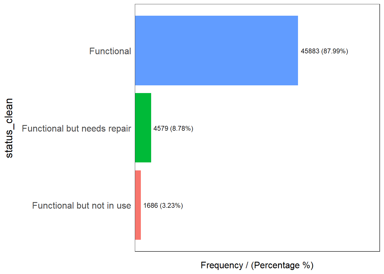
status_clean frequency percentage cumulative_perc
1 Functional 45883 87.99 87.99
2 Functional but needs repair 4579 8.78 96.77
3 Functional but not in use 1686 3.23 100.00freq(data = wp_nonfunctional,
input = 'status_clean')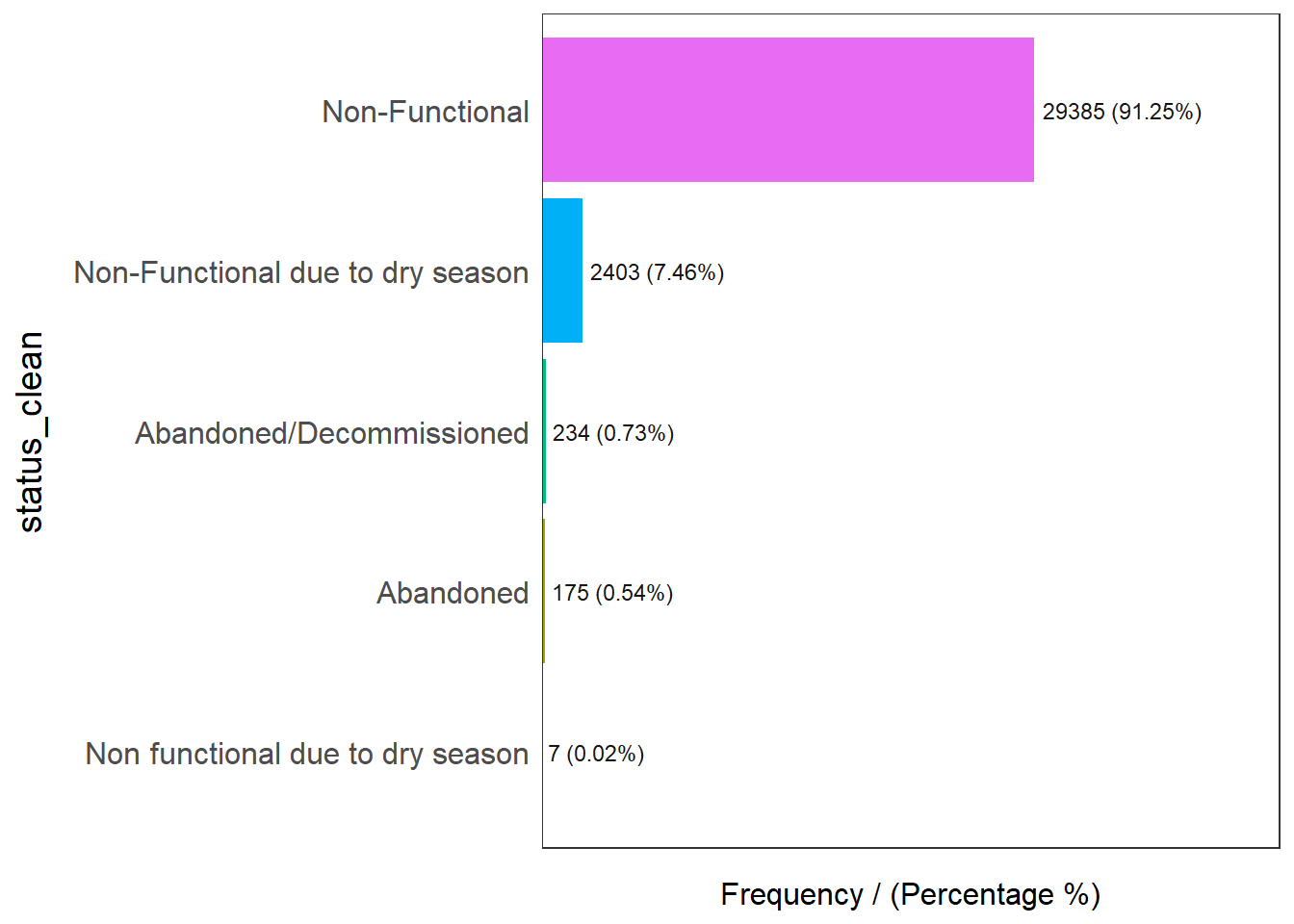
status_clean frequency percentage cumulative_perc
1 Non-Functional 29385 91.25 91.25
2 Non-Functional due to dry season 2403 7.46 98.71
3 Abandoned/Decommissioned 234 0.73 99.44
4 Abandoned 175 0.54 99.98
5 Non functional due to dry season 7 0.02 100.00freq(data = wp_unknown,
input = 'status_clean')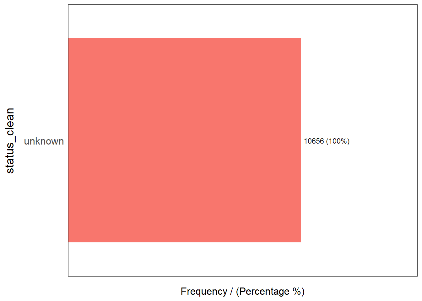
status_clean frequency percentage cumulative_perc
1 unknown 10656 100 1004.2 Performing Point-in-Polygon Count
Next, we want to find out the number of total, functional, nonfunctional and unknown water points in each LGA. This is performed in the following code chunk. First, it identifies the functional water points in each LGA by using st_intersects() of sf package. Next, length() is used to calculate the number of functional water points that fall inside each LGA.
NGA_wp <- NGA %>%
mutate(`total_wp` = lengths(
st_intersects(NGA, wp_sf_nga))) %>%
mutate(`wp_functional` = lengths(
st_intersects(NGA, wp_functional))) %>%
mutate(`wp_nonfunctional` = lengths(
st_intersects(NGA, wp_nonfunctional))) %>%
mutate(`wp_unknown` = lengths(
st_intersects(NGA, wp_unknown)))Notice that four new derived fields have been added into NGA_wp sf data.frame.
4.3 Visualing attributes by using statistical graphs
In this code chunk below, appropriate functions of ggplot2 package is used to reveal the distribution of total water points by LGA in histogram.
ggplot(data = NGA_wp,
aes(x = total_wp)) +
geom_histogram(bins=20,
color="black",
fill="light blue") +
geom_vline(aes(xintercept=mean(
total_wp, na.rm=T)),
color="red",
linetype="dashed",
size=0.8) +
ggtitle("Distribution of total water points by LGA") +
xlab("No. of water points") +
ylab("No. of\nLGAs") +
theme(axis.title.y=element_text(angle = 0))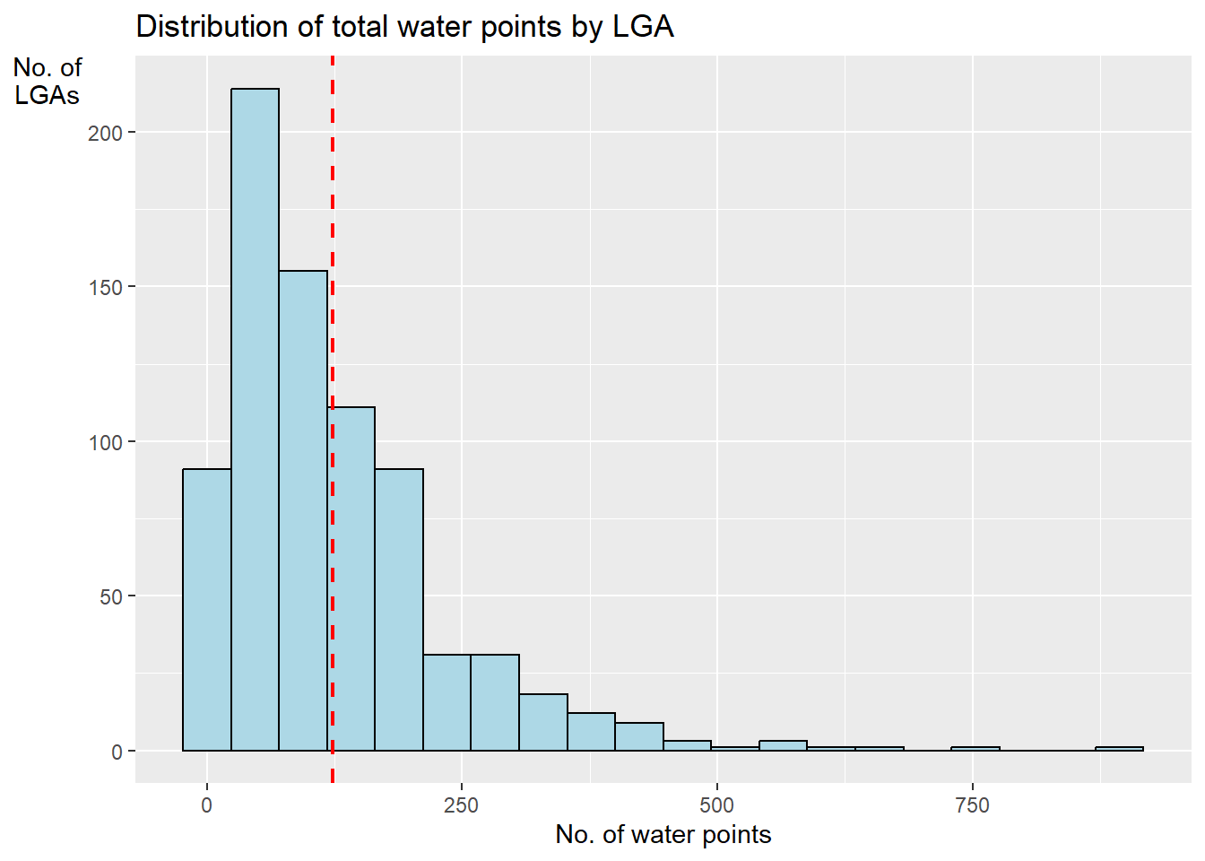
5 Exploratory Spatial Data Analysis (ESDA)
5.1 Basic Choropleth Mapping
5.2.1 Visualising Distribution of Functional Water Point by LGA
tmap_mode("view")
p1 <- tm_shape(NGA_wp) +
tm_fill("wp_functional",
n = 10,
style = "equal",
palette = "Blues") +
tm_borders(lwd = 0.1,
alpha = 1) +
tm_layout(main.title = "Distribution of functional water point by LGAs",
legend.outside = FALSE)
p1tmap_mode('plot')5.2.2 Visualising Distribution of Functional Water Point by LGA
tmap_mode("view")
p2 <- tm_shape(NGA_wp) +
tm_fill("wp_nonfunctional",
n = 10,
style = "equal",
palette = "Blues") +
tm_borders(lwd = 0.1,
alpha = 1) +
tm_layout(main.title = "Distribution of nonfunctional water point by LGAs",
legend.outside = FALSE)
p2tmap_mode('plot')5.2 Spatial Patterns from Kernel Density Maps
The advantage of kernel density map over point map: - better visualisation - summarises information of small zones compared to other zones
6 Second-order Spatial Point Patterns Analysis
Spatial Point Pattern Analysis is the evaluation of the pattern or distribution, of a set of points on a surface, using appropriate functions of spatstat. The point can be location of:
- events such as crime, traffic accident and disease onset, or
- business services (coffee and fastfood outlets) or facilities such as childcare and eldercare.
6.1 Spatial Data Wrangling
pacman::p_load(maptools, raster, spatstat)6.1.1 Mapping the Geospatial data sets
This step is useful for us to plot a map to show their spatial patterns.
tm_shape(wp_nonfunctional)+
tm_dots()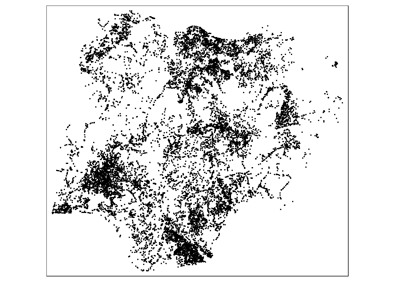
tmap_mode('plot')Reminder: Always remember to switch back to plot mode after the interactive map. This is because, each interactive mode will consume a connection. You should also avoid displaying excessive numbers of interactive maps (i.e. not more than 10) in one RMarkdown document when publish on Netlify.
6.2 Geospatial Data Wrangling
6.2.1 Converting sf data frames to sp’s Spatial* class
The code chunk below uses as_Spatial() of sf package to convert the three geospatial data from simple feature data frame to sp’s Spatial* class.
functional_sp <- as_Spatial(wp_functional)
nonfunctional_sp <- as_Spatial(wp_nonfunctional)functional_spclass : SpatialPointsDataFrame
features : 52148
extent : 29322.63, 1218553, 33758.37, 1092629 (xmin, xmax, ymin, ymax)
crs : +proj=tmerc +lat_0=4 +lon_0=8.5 +k=0.99975 +x_0=670553.98 +y_0=0 +a=6378249.145 +rf=293.465 +towgs84=-92,-93,122,0,0,0,0 +units=m +no_defs
variables : 1
names : status_clean
min values : Functional
max values : Functional but not in use nonfunctional_spclass : SpatialPointsDataFrame
features : 32204
extent : 28907.91, 1209690, 33736.93, 1092883 (xmin, xmax, ymin, ymax)
crs : +proj=tmerc +lat_0=4 +lon_0=8.5 +k=0.99975 +x_0=670553.98 +y_0=0 +a=6378249.145 +rf=293.465 +towgs84=-92,-93,122,0,0,0,0 +units=m +no_defs
variables : 1
names : status_clean
min values : Abandoned
max values : Non functional due to dry season Notice that the geospatial data have been converted into their respective sp’s Spatial* classes now.
6.2.2 Converting the generic sp format into spatstat’s ppp format
Now, we will use as.ppp() function of spatstat to convert the spatial data into spatstat’s ppp object format.
functional_ppp <-as(functional_sp, "ppp")
functional_pppMarked planar point pattern: 52148 points
marks are of storage type 'character'
window: rectangle = [29322.6, 1218553.3] x [33758.4, 1092628.9] unitsnonfunctional_ppp <-as(nonfunctional_sp, "ppp")
nonfunctional_pppMarked planar point pattern: 32204 points
marks are of storage type 'character'
window: rectangle = [28907.9, 1209690] x [33736.9, 1092882.6] unitsNow, let us plot functional_ppp and examine the difference.
plot(functional_ppp)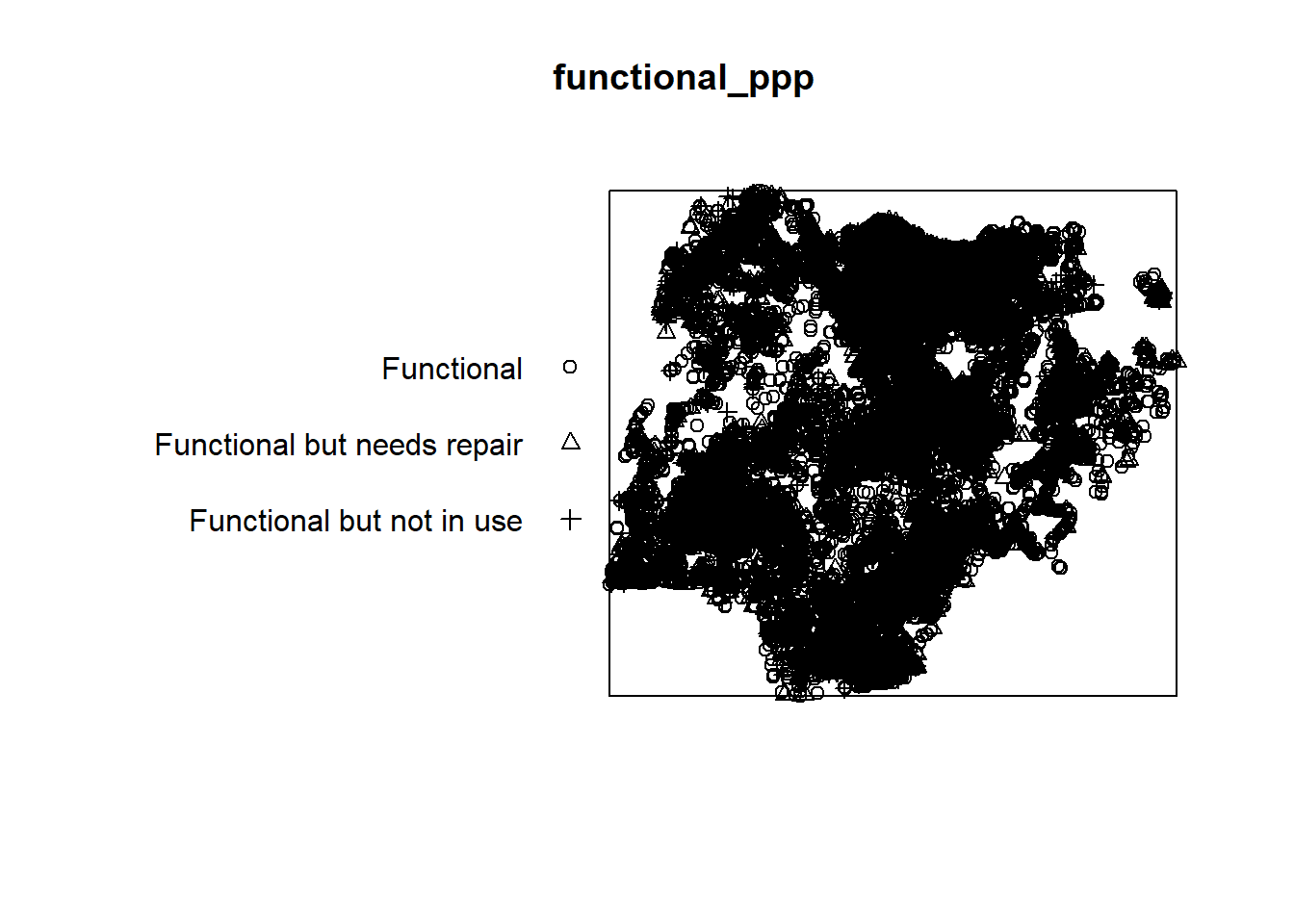
You can take a quick look at the summary statistics of the newly created ppp object by using the code chunk below.
summary(functional_ppp)Marked planar point pattern: 52148 points
Average intensity 4.141224e-08 points per square unit
Coordinates are given to 2 decimal places
i.e. rounded to the nearest multiple of 0.01 units
marks are of type 'character'
Summary:
Length Class Mode
52148 character character
Window: rectangle = [29322.6, 1218553.3] x [33758.4, 1092628.9] units
(1189000 x 1059000 units)
Window area = 1.25924e+12 square units6.3 Analysing Spatial Point Process Using L-Function
In this section, you will learn how to compute L-function estimation by using Lest() of spatstat package. You will also learn how to perform monta carlo simulation test using envelope() of spatstat package.
6.3.1 Functional Water Point
6.3.1.1 Computing L-Function Estimation
L_f = Lest(functional_ppp, correction = "Ripley")
plot(L_f, . -r ~ r,
ylab= "L(d)-r", xlab = "d(m)")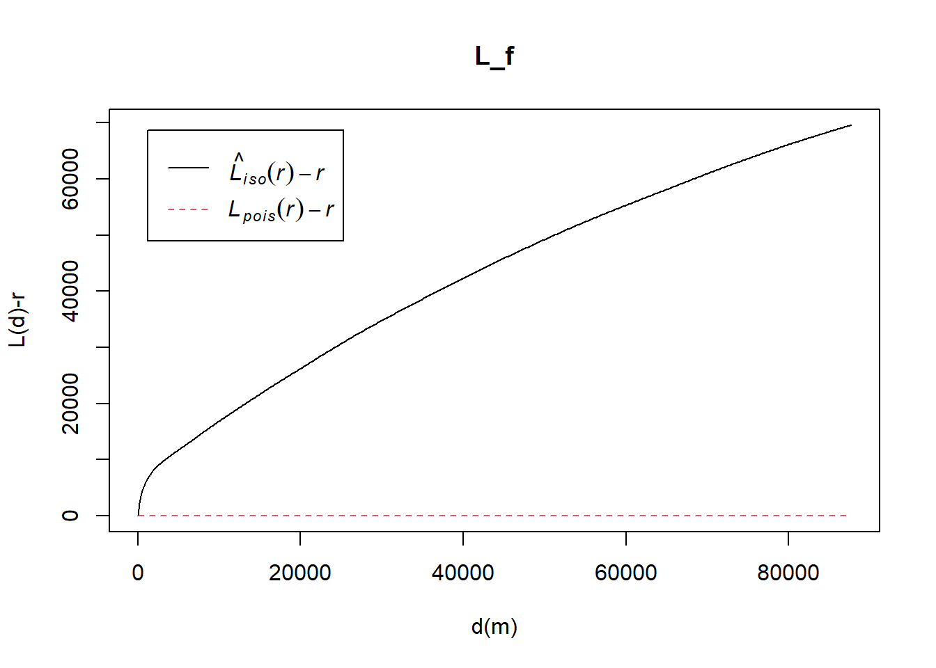
The plot above reveals that there is a sign that the distribution of Functional Water Point are not randomly distributed. However, a hypothesis test is required to confirm the observation statistically.
6.3.1.2 Performing Complete Spatial Randomness Test
To confirm the observed spatial patterns above, a hypothesis test will be conducted. The hypothesis and test are as follows:
Ho = The distribution of Functional Water Point are randomly distributed.
H1= The distribution of Functional Water Point are not randomly distributed.
The null hypothesis will be rejected if p-value is smaller than alpha value of 0.001.
Monte Carlo test with L-function.
L_f.csr = envelope(functional_ppp, Lest, nsim = 39, rank = 1, glocal=TRUE)Generating 39 simulations of CSR ...
1, 2, 3, 4, 5, 6, 7, 8, 9, 10, 11, 12, 13, 14, 15, 16, 17, 18, 19, 20, 21, 22, 23, 24, 25, 26, 27, 28, 29, 30, 31, 32, 33, 34, 35, 36, 37, 38, 39.
Done.plot(L_f.csr, . - r ~ r, xlab="d", ylab="L(d)-r")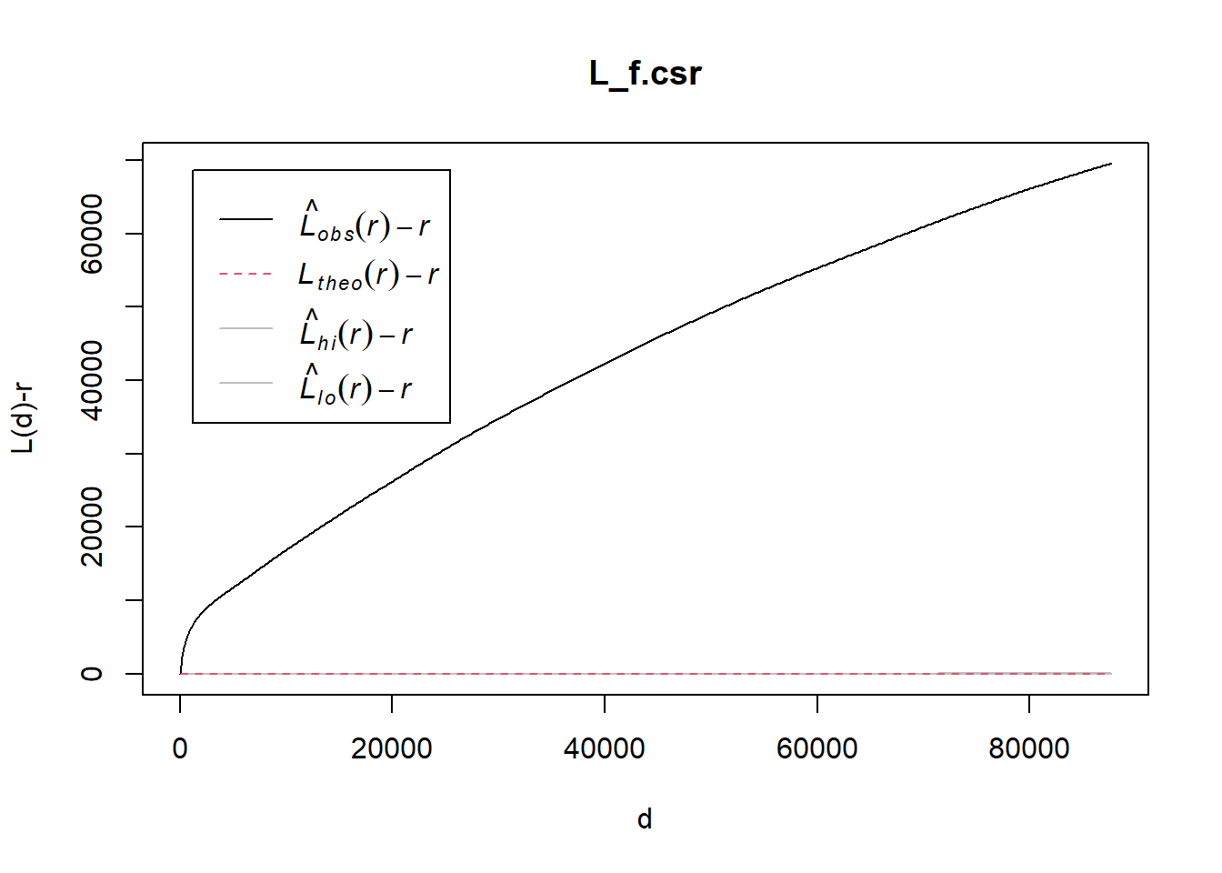
The plot above reveals that the are signs that the distribution of Functional Water Point are not randomly distributed. Unfortunately, we failed to reject the null hypothesis because the empirical k-cross line is within the envelop of the 95% confident interval.
6.3.2 Non-Functional Water Point
6.3.2.1 Computing L-Function Estimation
L_nf = Lest(nonfunctional_ppp, correction = "Ripley")
plot(L_nf, . -r ~ r,
ylab= "L(d)-r", xlab = "d(m)")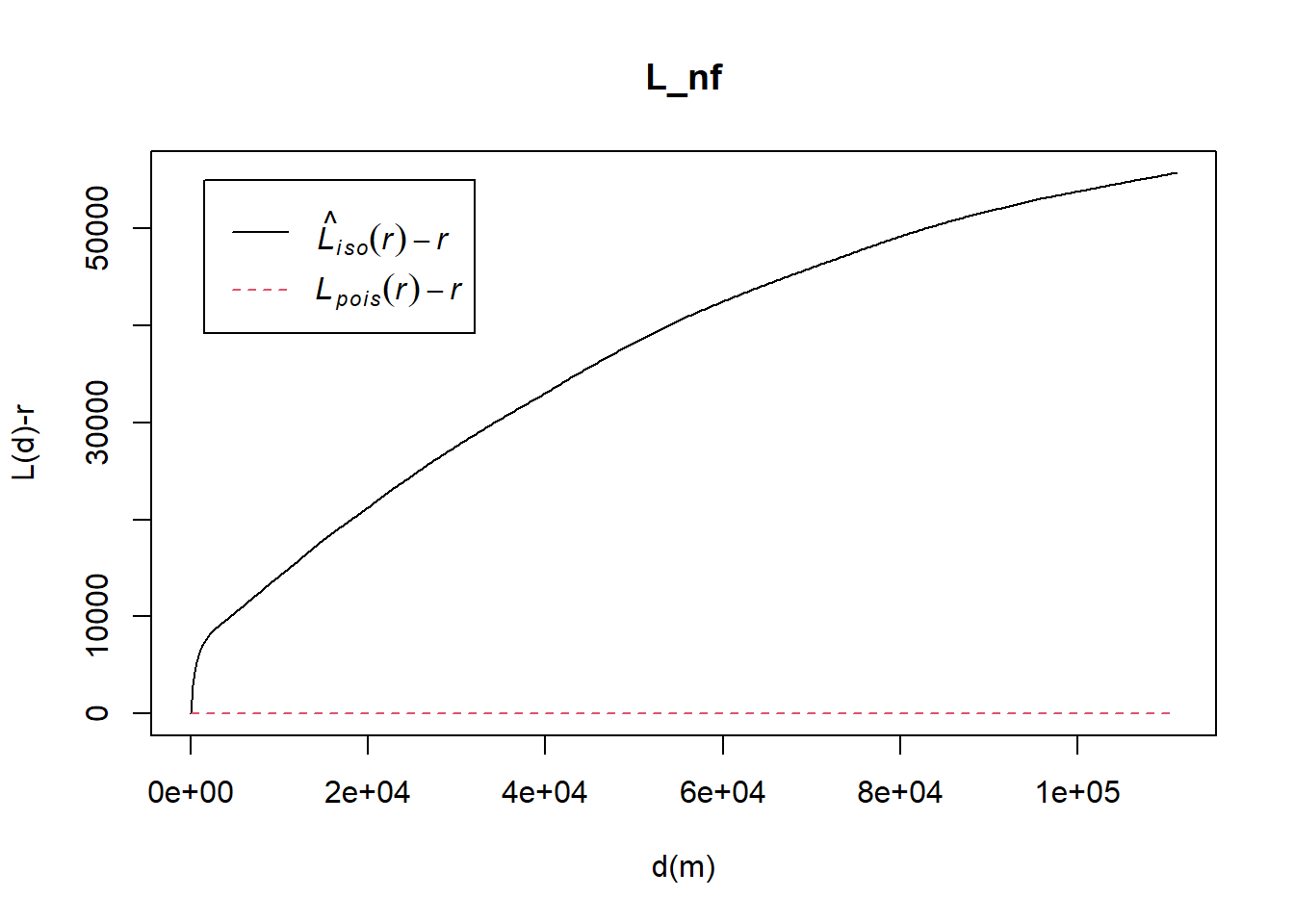
The plot above reveals that there is a sign that the distribution of Non-Functional Water Point are not randomly distributed. However, a hypothesis test is required to confirm the observation statistically.
6.3.2.2 Performing Complete Spatial Randomness Test
To confirm the observed spatial patterns above, a hypothesis test will be conducted. The hypothesis and test are as follows:
Ho = The distribution of Non-Functional Water Point are randomly distributed.
H1= The distribution of Non-Functional Water Point are not randomly distributed.
The null hypothesis will be rejected if p-value is smaller than alpha value of 0.001.
Monte Carlo test with L-function.
L_nf.csr = envelope(nonfunctional_ppp, Lest, nsim = 39, rank = 1, glocal=TRUE)Generating 39 simulations of CSR ...
1, 2, 3, 4, 5, 6, 7, 8, 9, 10, 11, 12, 13, 14, 15, 16, 17, 18, 19, 20, 21, 22, 23, 24, 25, 26, 27, 28, 29, 30, 31, 32, 33, 34, 35, 36, 37, 38, 39.
Done.plot(L_nf.csr, . - r ~ r, xlab="d", ylab="L(d)-r")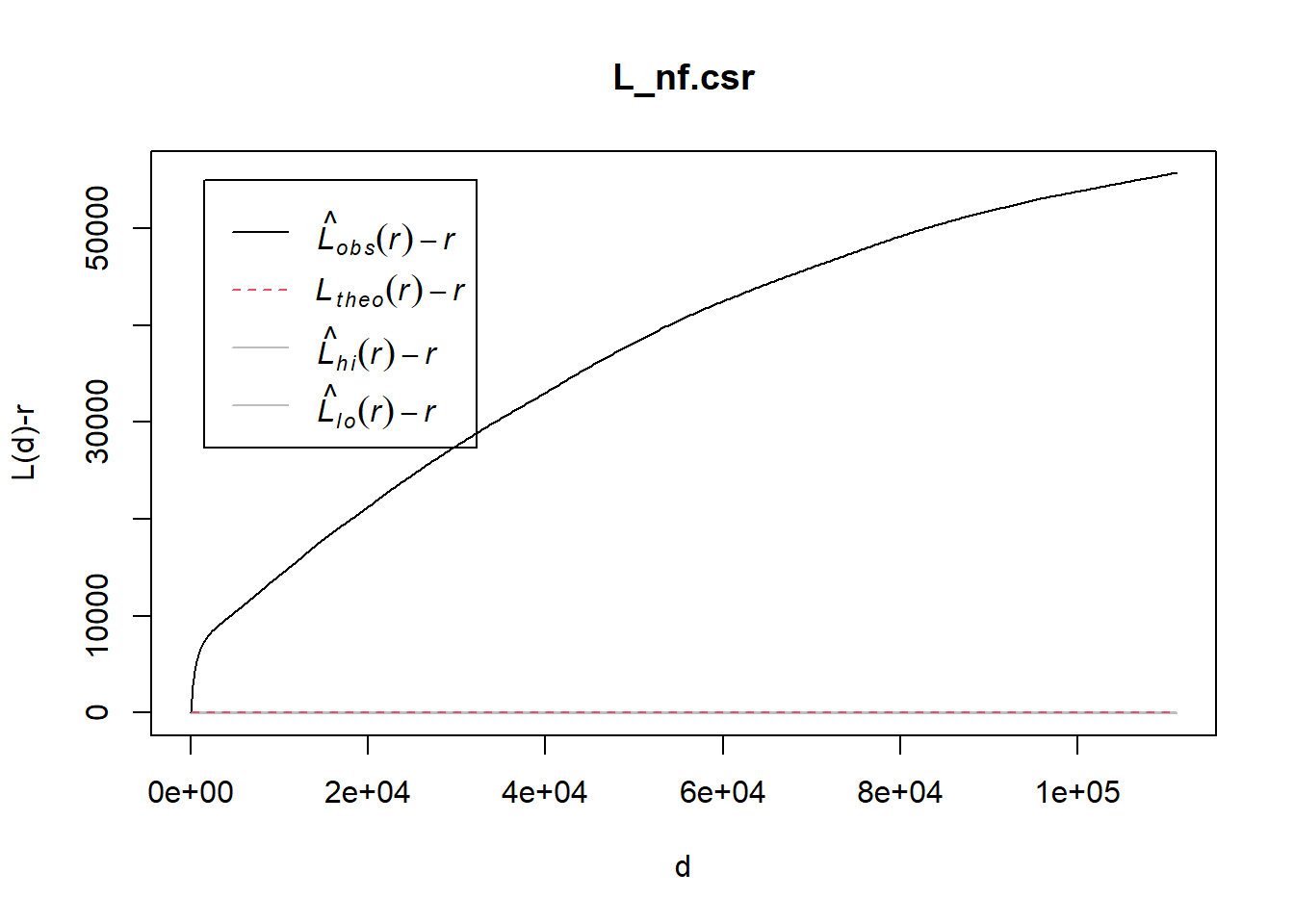
The plot above reveals that the are signs that the distribution of Non-Functional Water Point are not randomly distributed. Unfortunately, we failed to reject the null hypothesis because the empirical k-cross line is within the envelop of the 95% confident interval.
7 Spatial Correlation Analysis
In this section, we will confirm statistically if the spatial distribution of functional and non-functional water points are independent from each other.
7.1 Local Colocation Quotient Analysis (LCLQ)
7.1.1 Visualising the sf layers
Using the appropriate functions of tmap, we will be able to view the functional and non-functional water points on a single map.
tmap_mode("view")
tm_shape(NGA_wp) +
tm_polygons() +
tm_shape(wp_sf_nga)+
tm_dots(col = "status_clean",
size = 0.01,
border.col = "black",
border.lwd = 0.5) +
tm_view(set.zoom.limits = c(5, 16))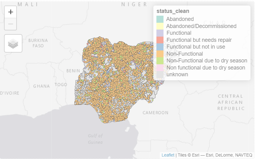
Notice that there are many categories for water point. For this exercise, we will have to combine all functional water point and non-functional water point into their own categories.
First, we will duplicate status_clean column.
wp_sf_nga$category <- wp_sf_nga$status_clean
wp_sf_ngaSimple feature collection with 95008 features and 2 fields
Geometry type: POINT
Dimension: XY
Bounding box: xmin: 28907.91 ymin: 33736.93 xmax: 1293293 ymax: 1092883
Projected CRS: Minna / Nigeria Mid Belt
# A tibble: 95,008 × 3
status_clean Geometry category
* <chr> <POINT [m]> <chr>
1 unknown (297874.6 441473.8) unknown
2 Functional (128394.3 330487.9) Functional
3 unknown (607559.4 274905.5) unknown
4 unknown (576523.1 301556.6) unknown
5 unknown (578321.7 307339.8) unknown
6 unknown (590994.2 326738.8) unknown
7 unknown (597909.2 333608.5) unknown
8 unknown (724171.9 367609.1) unknown
9 unknown (737994.1 350616.5) unknown
10 unknown (749790.1 354304.6) unknown
# … with 94,998 more rowsNext, we will have to change the value of “Functional but not in use” and “Functional but needs repair” into Functional.
wp_sf_nga$category[wp_sf_nga$category == "Functional but not in use"] <- "Functional"
wp_sf_nga$category[wp_sf_nga$category == "Functional but needs repair"] <- "Functional"Next, we will do the same for Non-functional.
wp_sf_nga$category[wp_sf_nga$category == "Abandoned/Decommissioned"] <- "Non-Functional"
wp_sf_nga$category[wp_sf_nga$category == "Abandoned"] <- "Non-Functional"
wp_sf_nga$category[wp_sf_nga$category == "Non-Functional due to dry season"] <- "Non-Functional"
wp_sf_nga$category[wp_sf_nga$category == "Non functional due to dry season"] <- "Non-Functional"We will run tmap again to view the data.
tmap_mode("view")
tm_shape(NGA_wp) +
tm_polygons() +
tm_shape(wp_sf_nga)+
tm_dots(col = "category",
size = 0.01,
border.col = "black",
border.lwd = 0.5) +
tm_view(set.zoom.limits = c(5, 16))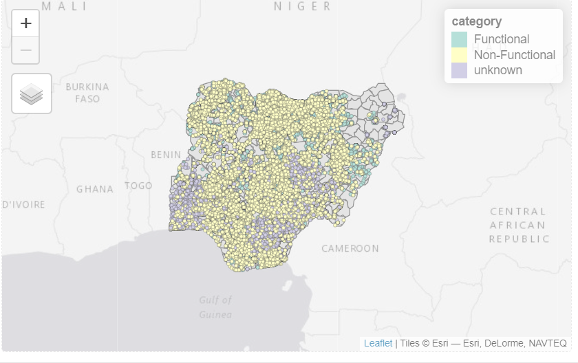
7.1.2 Preparing nearest Neighbours List
In the code chunk below, st_knn() of sfdep package is used to determine the k (i.e. 6) nearest neighbours for given point geometry.
nb <- include_self(
st_knn(st_geometry(wp_sf_nga), 6))7.1.3 Computing Kernal Weights
In the code chunk below, st_kernel_weights() of sfdep package is used to derive a weights list by using a kernel function.
wt <- st_kernel_weights(nb,
wp_sf_nga,
"gaussian",
adaptive = TRUE)For this to work: - an object of class nb e.g. created by using either st_contiguity() or st_knn() is required. - The supported kernel methods are: “uniform”, “gaussian”, “triangular”, “epanechnikov”, or “quartic”.
7.1.4 Preparing the Vector List
To compute LCLQ by using sfdep package, the reference point data must be in either character or vector list. The code chunks below are used to prepare two vector lists. One of Functional and for Non-Functional and are called A and B respectively.
functional <- wp_sf_nga %>%
filter(category == "Functional")
A <- functional$categorynon_functional <- wp_sf_nga %>%
filter(category == "Non-Functional")
B <- non_functional$category